This pattern is designed to give you a quick ranking so you can isolate the top X of a subcategory in your workbook but also shows how you can promote this logic to be reusable and more scalable in the model layer.
Setup:
- Primary Category dimension (Country in this example)
- Secondary Category dimension (State in this example)
- Metric to rank with (User count in this example)
- Sort first on Primary, then secondary sort (shift+click) on the metric to get descending. These sort conditions must stay applied or the formula will not work.
Formula:
Add the following formula to the second row of the new calc. The offset reference will error if the formula is added to the first row.
Double-click to access edit mode in the cell, then input the formula:
=IF((ROW() = 1), 0, IF((A2 = A1), COUNTIF(A$1:A1, A2), 0)) + 1
Output
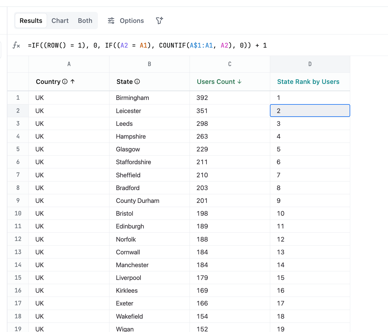
And you can see it detects the point at which UK ends and USA begins (why the sort is required for this to work)

Getting Top 10

Just filter on your rank calculation for <11 and boom, you have top 10 subcategories of each primary category without any modeling ![]()
Convert the calc for more robust analysis
And, if you want to a little further you can easily do even more cool stuff like this:

- From the workbook tab Model > Save as Query View then choose “Use in Query
 ” in the top right
 - In the field picker on state, select Aggregates > List from the field options
- Select State Rank, and State List, then pivot on Country to get a nice table of your top 10s